y⁺ explained: getting the near-wall mesh right

Wall shear stress, heat transfer and the onset of separation are all decided in a thin layer next to the wall. How the mesh treats that layer matters more than almost any other meshing choice, and y⁺ is the number used to describe it. This article explains what y⁺ measures, which values to aim for, and how to estimate the first-cell height before meshing.

The law of the wall

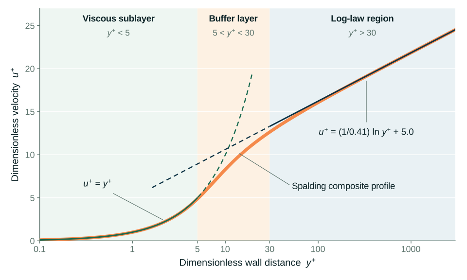
Close to a wall, the mean velocity of a turbulent boundary layer collapses onto a near-universal profile when scaled with the friction velocity u_τ = √(τ_w / ρ), where τ_w is the wall shear stress. The dimensionless wall distance and velocity are

y⁺ = y u_τ / ν, and u⁺ = u / u_τ

The inner part of the boundary layer then has three zones:

• Viscous sublayer, y⁺ below about 5. Viscous stress dominates and the profile is linear: u⁺ = y⁺.
• Buffer layer, y⁺ from about 5 to 30. Viscous and turbulent stresses are comparable, turbulence production peaks, and neither simple law fits.
• Log layer, y⁺ above about 30. Turbulent stress dominates and u⁺ = (1/κ) ln y⁺ + B, with κ ≈ 0.41 and B ≈ 5.0 to 5.2.

The linear and log laws intersect at y⁺ ≈ 11. The upper end of the log layer depends on Reynolds number, so the figure of 300 usually quoted is a guideline, not a physical limit.

Two meshing strategies

Wall-resolved. The first cell sits in the viscous sublayer, at y⁺ ≈ 1, and the turbulence model is integrated to the wall. This is what k-ω SST, Spalart–Allmaras and transition models are designed for, and it is the appropriate choice when wall heat transfer, skin friction or the separation point matter.

Wall functions. The first cell sits in the log layer, at 30 < y⁺ < 300, and the solver bridges the sublayer with the log law. This saves many cells at high Reynolds number, but it assumes an equilibrium boundary layer. That assumption weakens in separation, strong pressure gradients, impingement and buoyancy-driven flow.

The awkward zone is the buffer layer. A first cell at y⁺ of 5 to 30 is too coarse for a wall-resolved model and too fine for a standard wall function, which then applies the log law where it does not hold. Blended or "all-y⁺" treatments in current solvers reduce the sensitivity but do not remove the error.

Estimating the first-cell height

y⁺ depends on the solution, so it cannot be known before the run. A flat-plate correlation gives an estimate good enough for the first mesh.

1. Compute the Reynolds number from the free-stream velocity and a reference length: Re_x = ρ U_∞ x / μ.
2. Estimate the skin-friction coefficient, for example with Schlichting's correlation for a turbulent flat plate: C_f = (2 log₁₀ Re_x − 0.65)^−2.3. The simpler power law C_f ≈ 0.058 Re_x^−0.2 gives similar values.
3. Wall shear stress: τ_w = ½ C_f ρ U_∞².
4. Friction velocity: u_τ = √(τ_w / ρ).
5. Wall distance for the target y⁺: y = y⁺ ν / u_τ.

Take air (ρ = 1.2 kg/m³, μ = 1.8 × 10⁻⁵ Pa·s) at 20 m/s over a 1 m length. Then Re_x ≈ 1.3 × 10⁶, C_f ≈ 0.0036, τ_w ≈ 0.86 Pa and u_τ ≈ 0.84 m/s. A target of y⁺ = 1 gives y ≈ 0.018 mm; a target of y⁺ = 50 gives y ≈ 0.9 mm.

Two cautions. First, check how your solver defines y. Cell-centred finite-volume codes evaluate y⁺ at the centroid of the first cell, so the first-cell height is twice the value of y from step 5. Second, this is a flat-plate estimate. Real y⁺ is higher where the flow accelerates and lower near stagnation and separation. For internal flows, use the bulk velocity, the hydraulic diameter and a pipe-friction correlation.

Inflation layers and growth ratio

The layers above the first cell must carry the mesh smoothly through the whole boundary layer.

• Growth ratio. Keep the ratio between successive layer heights at about 1.1 to 1.2 for wall-resolved meshes; up to about 1.3 is often tolerated with wall functions. These are working guidelines, not hard limits.
• Total thickness. The layers should span the boundary layer. For a turbulent flat plate, δ ≈ 0.37 x / Re_x^0.2 at a distance x from the leading edge, which is about 22 mm at the end of the plate in the example above.
• Layer count. For first height h₁, ratio r and N layers, the total is h₁ (r^N − 1) / (r − 1). Covering 22 mm from a 0.036 mm first cell at r = 1.2 takes roughly 27 layers.
• Transition to the core mesh. The last layer should be similar in size to the adjacent core cells. A sudden jump in cell volume there degrades accuracy.

Checking y⁺ after the run

Treat y⁺ as a result to be checked, not a setting.

• Plot y⁺ over every wall that matters, and look at the range and distribution, not just an area average.
• With wall functions, look for patches that have dropped into the buffer layer or below.
• y⁺ falls towards zero wherever wall shear vanishes, as at separation and reattachment. A low value there says nothing about mesh quality.
• A good y⁺ does not show that the boundary layer has enough layers, or that the streamwise spacing is adequate. Only a refinement study shows that; see mesh independence and the Grid Convergence Index.

If the values are off target, rescale the first-layer height by the ratio of target to achieved y⁺ and rerun. The choice of wall treatment is also tied to the turbulence model, covered in RANS, LES or DES?

How CFD Pro can help

CFD Pro provides CFD and thermal simulation services, supporting clients from problem definition through to verified results and reporting. Near-wall meshing is part of that work. To discuss a meshing strategy or a complete study, send us a project brief.